
Problem: Spatial Pattern Analysis involves using a variety of GIS spatial analysis tools to analyze patterns and identify clusters in your data. GIS Analysts are required to have a good understanding of the various spatial analysis tools in esri ArcGIS and when to apply them for different types of spatial pattern analysis. There are many different tools in ArcGIS that build on each other in order to dig deeper into the data to understand the statistical significance of clustering patterns and hot spots. In this example some ArcGIS tools are discussed for performing spatial pattern analysis such as:
- When and how to performing a nearest neighbor spatial analysis and calculating Nearest Neighbor Index, Z-Score, and determining probability confidence intervals.
- When and how to performing a Getis-Ord General G high/low clustering pattern analysis and understanding the concepts of spatial relationships that data features have and when to utilize inverse distance squared, fixed distance band, and zone of indifference settings.
- When and how to check for multi-distance clustering using Ripley’s K function that examines the counts of neighboring features at several distances and plotting the different K values between the actual dataset and the hypothetical dataset to identify the distance where the most pronounced spatial clustering occurs.
- When and how to measure spatial autocorrelation using the Moran’s I index to determine if the data are clustered, random, or dispersed.
- Once statistical significance is established how to use tools for pinpointing the location of clustering patterns and identifying hotspots, cold spots, and outliers.
As an example to demonstrate an understanding of these concepts three different data sets provided from clients who have questions about their data they have collected were answered. These spatial analysis questions include:
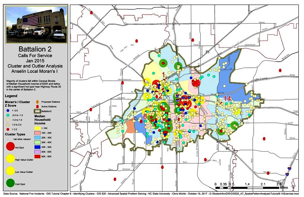
- For an Emergency Response Service Company analyze calls for emergency service to identify if calls for service are clustered or random, whether false alarm calls tend to cluster from any particular area within their Batallion 2 district and whether the highest priority emergency calls tend to cluster in certain areas such as near highways or dangerous intersections.
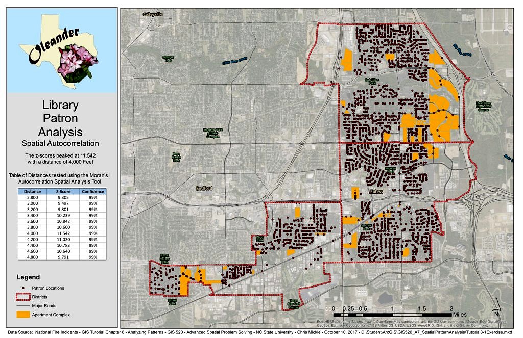
- For a community in Texas, examine the locations of library customers to determine the density of library patrons per block and identify the distance at which the most significant clustering occurs.
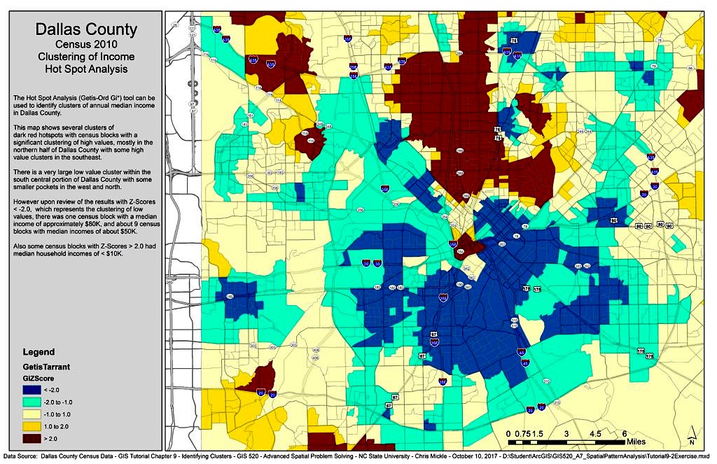
- For Dallas County assess the median household income census data to determine if there is clustering where does the clustering of income values occur in the high and low median income ranges.
Analysis Procedures: To answer the questions above the appropriate data needed to be obtained to address each problem. These data were provided by each client looking for their questions about their data to be answered. The data was reviewed and explored using ArcMap 10.4.1 in order to identify the data elements and data types contained. Depending on the information provided, and question to be answered, the ArcGIS spatial analysis tool or tools was chosen based on where in the spatial analysis process we were and the type of map was needed to display the information and refine the results.
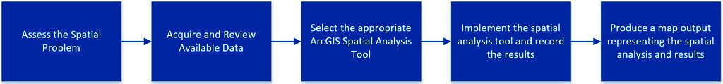
The methods implemented following the high level process for performing spatial pattern analysis, identifying clustering and hot spot analysis is overall the same for each problem. However different tools and questions were answered. Unique methods implemented for addressing each of the spatial analysis questions above are organized below.
Emergency Response Service Company Analysis
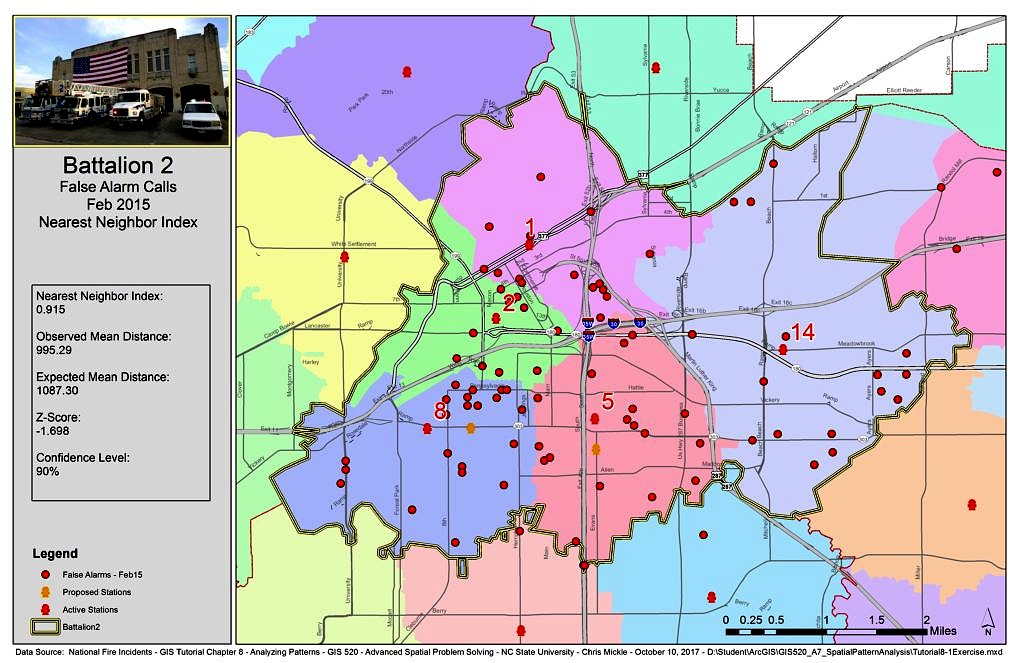
For analyzing patterns and to assess if EMS calls are clustered and where false alarm calls tend to be clustered data from the National Fire Incidents for February 2015 was analyzed. The Average Nearest Neighbor spatial pattern analysis tool was used in ArcMap 10.4.1 and the Nearest Neighbor index less than 1 was recorded indicating the calls are clustered.
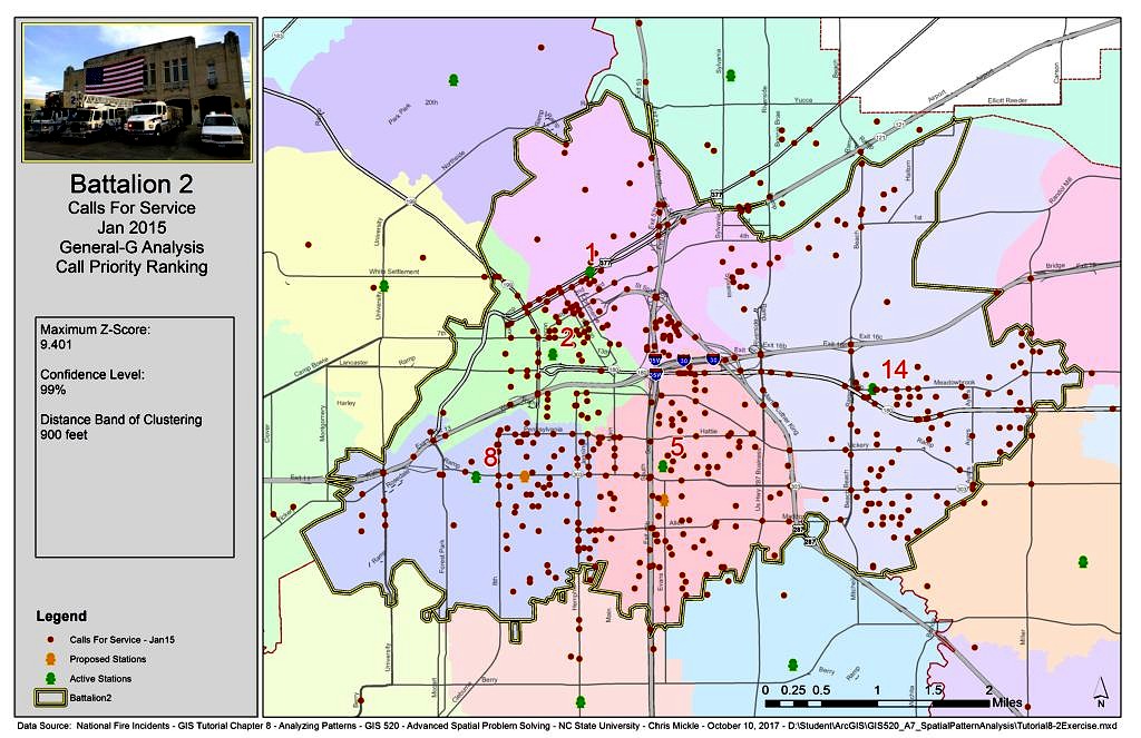
Once clustering was identified, the High/Low Clustering (Getis-Ord General G) tool was used to generate a Z-Score and determine whether calls ranked as high priority are clustered or if they are randomly distributed across the area and what is the distance band of the clustering. The General G Statistic measures how high or how low values associated within a specific distance are in comparison to those features outside a specified distance.
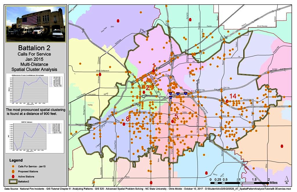
Another method for analyzing spatial patterns and clustering is to check for multi-distance spatial clustering of the January 2015 fire department calls for service data using the esri ArcGIS 10.4.1 Multi-Distance Spatial Cluster Analysis tool. This tool examines the counts of neighboring features at several distances and generates a hypothetical (Expected) random distribution to compare the actual (Observed) data to and then calculates the difference. These differences were then plotted graphically. The Ripley’s K function was then run again with the Confidence Envelope setting enabled for a number of permutations so the upper limit of the confidence envelope can be compared to the observed K.
Clustered data in certain areas are referred to as "Hot Spots". For identifying "Hot Spot" clusters, and outliers once statistical significance is established, the Cluster and Outlier Analysis (Anselin Local Morans I) tool in ArcMap 10.4.1 was used to assist the Battalion 2 EMS determine hot and cold spot clusters as they pertained to median household income areas. Based on the analysis it was concluded that the majority of EMS calls were clustered in Census blocks with a median income of $30K or less.
Library Patron Analysis
Spatial autocorrelation includes looking at both the feature locations and their attributes simultaneously. The Moran’s I index is calculated using the Spatial Autocorrelation (Moran’s I) tool in ArcMap 10.4.1. This tool was used for helping Oleander, Texas with their analysis of library patrons to determine if they are randomly distributed among city blocks. After examining all of the Z-Scores the NULL hypothesis that library patrons are randomly distributed was rejected as there is there is less than 1% likelihood that the clustered pattern is the result of a random chance.
Household Income Analysis
For Dallas County the Hot Spot Analysis (Getis-Ord Gi*) tool in ArcMap 10.4.1 was used to identify clusters of annual median income. Census blocks are symbolized with median income values and displayed high to low value clustering. Looking at the data closely revealed some outliers within the high and low clustered values.
Application and Reflection
The spatial pattern analysis and clustering tools are extremely useful when analyzing environmental data. Soil and groundwater contamination data are continuously collected and evaluated. Spatial pattern analysis tools help to evaluate our data sets and understand whether our data are clustered or randomly sampled representations of the conditions at study sites. This is especially important as soil or groundwater contamination data are modeled and plumes are identified. Plumes models include a visualization of data in areas where the model interpolates a concentration at a given point between known data points and the percent confidence of probability needs to be known. Spatial pattern analysis help us to identify clustered areas as hot spots but also recognize areas where data lack in order to appropriately weigh these different points and adjust our models for the areas where more data collection is needed or interpolate to determine the concentrations without hot spots or cold spots skewing these areas.
- Problem description: Soil and groundwater contamination data are collected by various parties for different reasons on properties that may have a contamination issue. Some of the reason's for collecting the data may be for understanding protection to drinking water, human health risks, and ecological risks. The data may be collected by a regulatory agency responsible for enforcing environmental laws and clean up standards or by third party investors performing due diligence research in order to purchase or divest a given property. A historical contamination site has a large data site that has been aggregated over several years in an environmental database. The sampling locations come from data providers with all of the various jurisdiction and business intents previously mentioned. Analyze the sampling locations of the entire data set to determine if the data are clustered or randomly dispersed as a clustered data set will indicate hot spots based on known concentration values in the result data set.
- Data needed: The sampling locations of all soil and groundwater data are needed in a single data set in a uniform spatial projection by media. The analysis of soil and groundwater sampling locations needs to be separate as the data are analyzed separately even thought they can inform contamination areas simultaneously.
- Analysis procedures: Use the Average Nearest Neighbor spatial pattern analysis tool in ArcMap 10.4.1 to determine if the Nearest Neighbor index is less than 1 and sampling locations are clustered.